
利用tensorboard调参
import os
import tensorflow as tf
import urllib

LOGDIR = '/tmp/mnist_tutorial/'
GITHUB_URL ='https://raw.githubusercontent.com/mamcgrath/TensorBoard-TF-Dev-Summit-Tutorial/master/'
LOGDIR = '/tmp/mnist_tutorial/'

### MNIST EMBEDDINGS ###
mnist = tf.contrib.learn.datasets.mnist.read_data_sets(train_dir=LOGDIR + 'data', one_hot=True)
### Get a sprite and labels file for the embedding projector ###
urllib.urlretrieve(GIST_URL + 'labels_1024.tsv', LOGDIR + 'labels_1024.tsv')
urllib.urlretrieve(GIST_URL + 'sprite_1024.png', LOGDIR + 'sprite_1024.png')


def conv_layer(input, size_in, size_out, name="conv"):
  #tf.name_scope creates namespace for operators in the default graph , places into group, easier to read
  #A graph maintains a stack of name scopes. A `with name_scope(...):`
  #statement pushes a new name onto the stack for the lifetime of the context.
  #Ops have names, name scopes group ops
  with tf.name_scope(name):
    w = tf.Variable(tf.truncated_normal([5, 5, size_in, size_out], stddev=0.1), name="W")
    b = tf.Variable(tf.constant(0.1, shape=[size_out]), name="B")
    conv = tf.nn.conv2d(input, w, strides=[1, 1, 1, 1], padding="SAME")
    act = tf.nn.relu(conv + b)
    #collect this data by attaching tf.summary.histogram ops to the gradient outputs and to the variable that holds weights, respectively.
    #visualize the the distribution of weights and biases
    tf.summary.histogram("weights", w)
    tf.summary.histogram("biases", b)
    tf.summary.histogram("activations", act)
    return tf.nn.max_pool(act, ksize=[1, 2, 2, 1], strides=[1, 2, 2, 1], padding="SAME")


def fc_layer(input, size_in, size_out, name="fc"):
  with tf.name_scope(name):
    w = tf.Variable(tf.truncated_normal([size_in, size_out], stddev=0.1), name="W")
    b = tf.Variable(tf.constant(0.1, shape=[size_out]), name="B")
    act = tf.nn.relu(tf.matmul(input, w) + b)
    tf.summary.histogram("weights", w)
    tf.summary.histogram("biases", b)
    tf.summary.histogram("activations", act)
    return act


def mnist_model(learning_rate, use_two_conv, use_two_fc, hparam):
  tf.reset_default_graph()
  sess = tf.Session()

  # Setup placeholders, and reshape the data
  x = tf.placeholder(tf.float32, shape=[None, 784], name="x")
  x_image = tf.reshape(x, [-1, 28, 28, 1])
  #Outputs a Summary protocol buffer with 3 images.
  tf.summary.image('input', x_image, 3)
  y = tf.placeholder(tf.float32, shape=[None, 10], name="labels")

  if use_two_conv:
    conv1 = conv_layer(x_image, 1, 32, "conv1")
    conv_out = conv_layer(conv1, 32, 64, "conv2")
  else:
    conv1 = conv_layer(x_image, 1, 64, "conv")
    conv_out = tf.nn.max_pool(conv1, ksize=[1, 2, 2, 1], strides=[1, 2, 2, 1], padding="SAME")

  flattened = tf.reshape(conv_out, [-1, 7 * 7 * 64])


  if use_two_fc:
    fc1 = fc_layer(flattened, 7 * 7 * 64, 1024, "fc1")
    #we want these embeeddings to visualize them later
    embedding_input = fc1
    embedding_size = 1024
    logits = fc_layer(fc1, 1024, 10, "fc2")
  else:
    embedding_input = flattened
    embedding_size = 7*7*64
    logits = fc_layer(flattened, 7*7*64, 10, "fc")
  with tf.name_scope("xent"):
    xent = tf.reduce_mean(
        tf.nn.softmax_cross_entropy_with_logits(
            logits=logits, labels=y), name="xent")
    #save that single number
    tf.summary.scalar("xent", xent)

  with tf.name_scope("train"):
    train_step = tf.train.AdamOptimizer(learning_rate).minimize(xent)

  with tf.name_scope("accuracy"):
    correct_prediction = tf.equal(tf.argmax(logits, 1), tf.argmax(y, 1))
    accuracy = tf.reduce_mean(tf.cast(correct_prediction, tf.float32))
    tf.summary.scalar("accuracy", accuracy)
  #Merges all summaries collected in the default graph
  summ = tf.summary.merge_all()

  #intiialize embedding matrix as 0s
  embedding = tf.Variable(tf.zeros([1024, embedding_size]), name="test_embedding")
  #give it calculated embedding
  assignment = embedding.assign(embedding_input)
  #initialize the saver
  # Add ops to save and restore all the variables.
  saver = tf.train.Saver()

  sess.run(tf.global_variables_initializer())
  #filewriter is how we write the summary protocol buffers to disk
  #writer = tf.summary.FileWriter(<some-directory>, sess.graph)
  writer = tf.summary.FileWriter(LOGDIR + hparam)
  writer.add_graph(sess.graph)

  ## Format: tensorflow/contrib/tensorboard/plugins/projector/projector_config.proto
  config = tf.contrib.tensorboard.plugins.projector.ProjectorConfig()
  ## You can add multiple embeddings. Here we add only one.
  embedding_config = config.embeddings.add()
  embedding_config.tensor_name = embedding.name
  embedding_config.sprite.image_path = LOGDIR + 'sprite_1024.png'
  embedding_config.metadata_path = LOGDIR + 'labels_1024.tsv'
  # Specify the width and height of a single thumbnail.
  embedding_config.sprite.single_image_dim.extend([28, 28])
  tf.contrib.tensorboard.plugins.projector.visualize_embeddings(writer, config)

  for i in range(2001):
    batch = mnist.train.next_batch(100)
    if i % 5 == 0:
      [train_accuracy, s] = sess.run([accuracy, summ], feed_dict={x: batch[0], y: batch[1]})
      #This method wraps the provided summary in an Event protocol buffer and adds it to the event file.
      writer.add_summary(s, i)
    if i % 500 == 0:
      sess.run(assignment, feed_dict={x: mnist.test.images[:1024], y: mnist.test.labels[:1024]})
      saver.save(sess, os.path.join(LOGDIR, "model.ckpt"), i)
    sess.run(train_step, feed_dict={x: batch[0], y: batch[1]})

def make_hparam_string(learning_rate, use_two_fc, use_two_conv):
  conv_param = "conv=2" if use_two_conv else "conv=1"
  fc_param = "fc=2" if use_two_fc else "fc=1"
  return "lr_{}_{}_{}".format(learning_rate, conv_param, fc_param)

def main():
  # You can try adding some more learning rates
  for learning_rate in [1E-3,1E-4]:

    # Include "False" as a value to try different model architectures
    for use_two_fc in [True,False]:
      for use_two_conv in [True,False]:
        # Construct a hyperparameter string for each one (example: "lr_1E-3,fc=2,conv=2)
        hparam = make_hparam_string(learning_rate, use_two_fc, use_two_conv)
        print('Starting run for %s' % hparam)

	# Actually run with the new settings
        mnist_model(learning_rate, use_two_fc, use_two_conv, hparam)


if __name__ == '__main__':
  main()
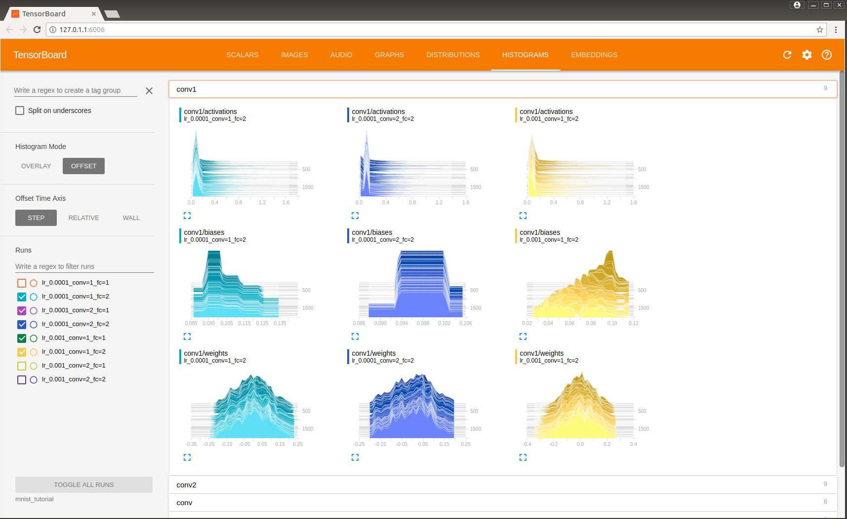
如何读懂tensorboard上的图示
上述代码建立了尝试不同learning rates和不同网络结构训练模型的结果
可以建立一个hyperparameter stringr然后在打开Board时指向上一层目录文件夹,这样就可以合并多个不同参数下的模型图表。
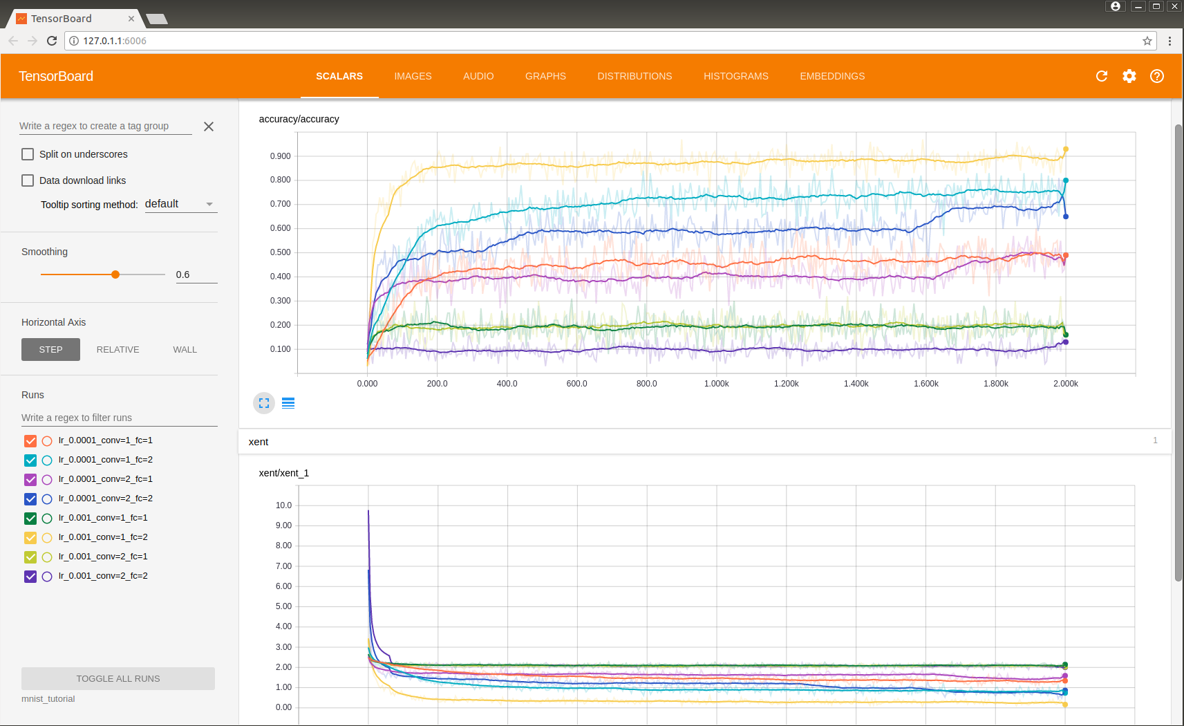
如图展示了不同参数下网络训练的结果,可见最好的结果是在参数lr=0.0001,conv=1,fc=2.可以用realtive查看不同模型所需训练时间,wall查看在何时训练的。
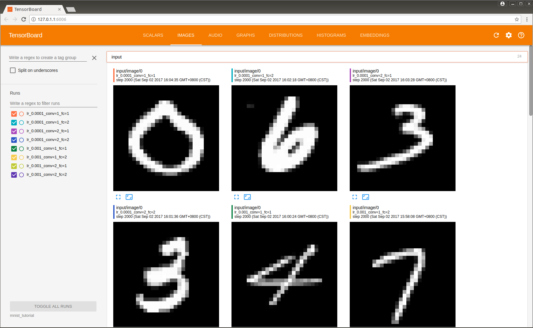
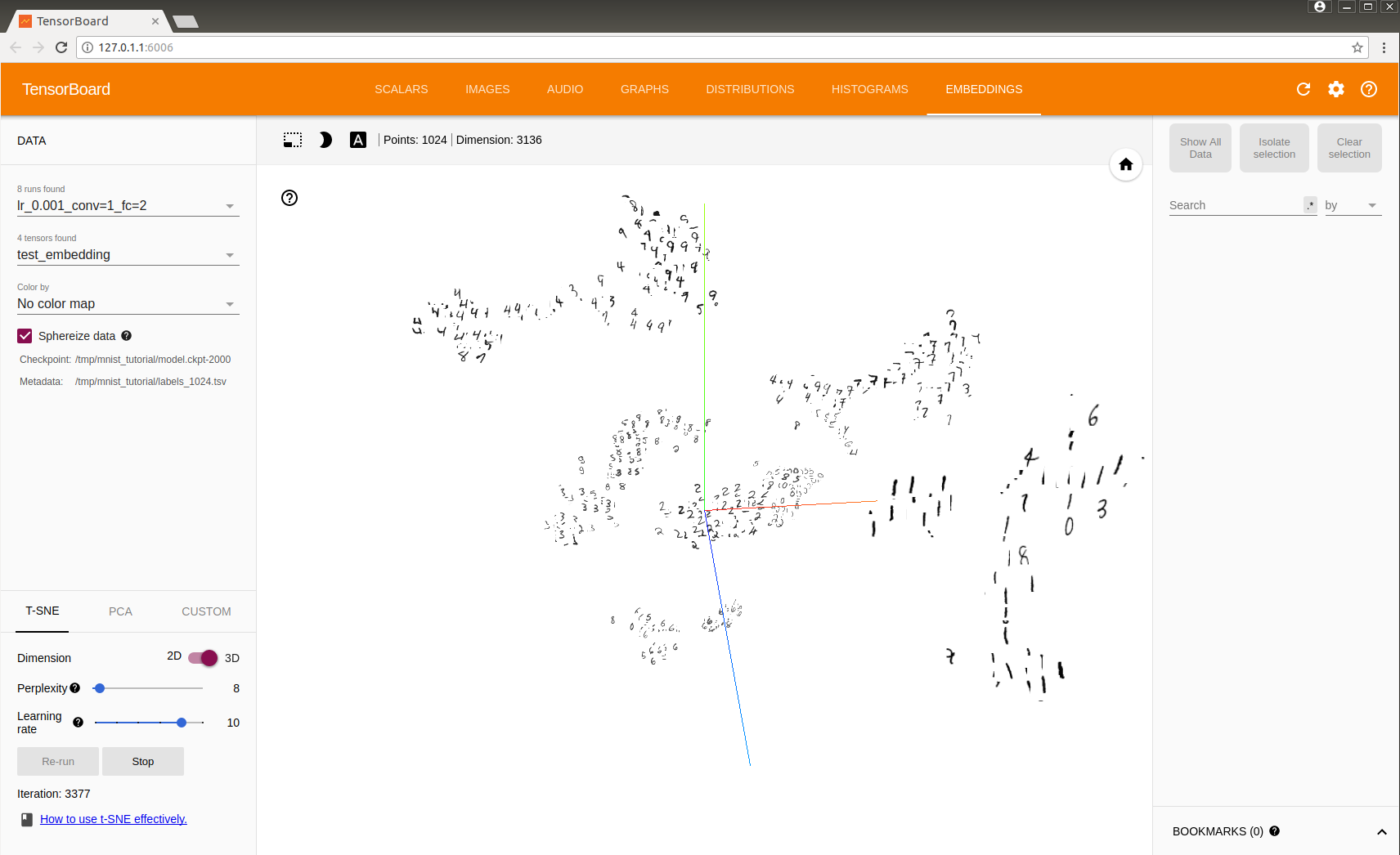
如图展示了不同模型的图片内容
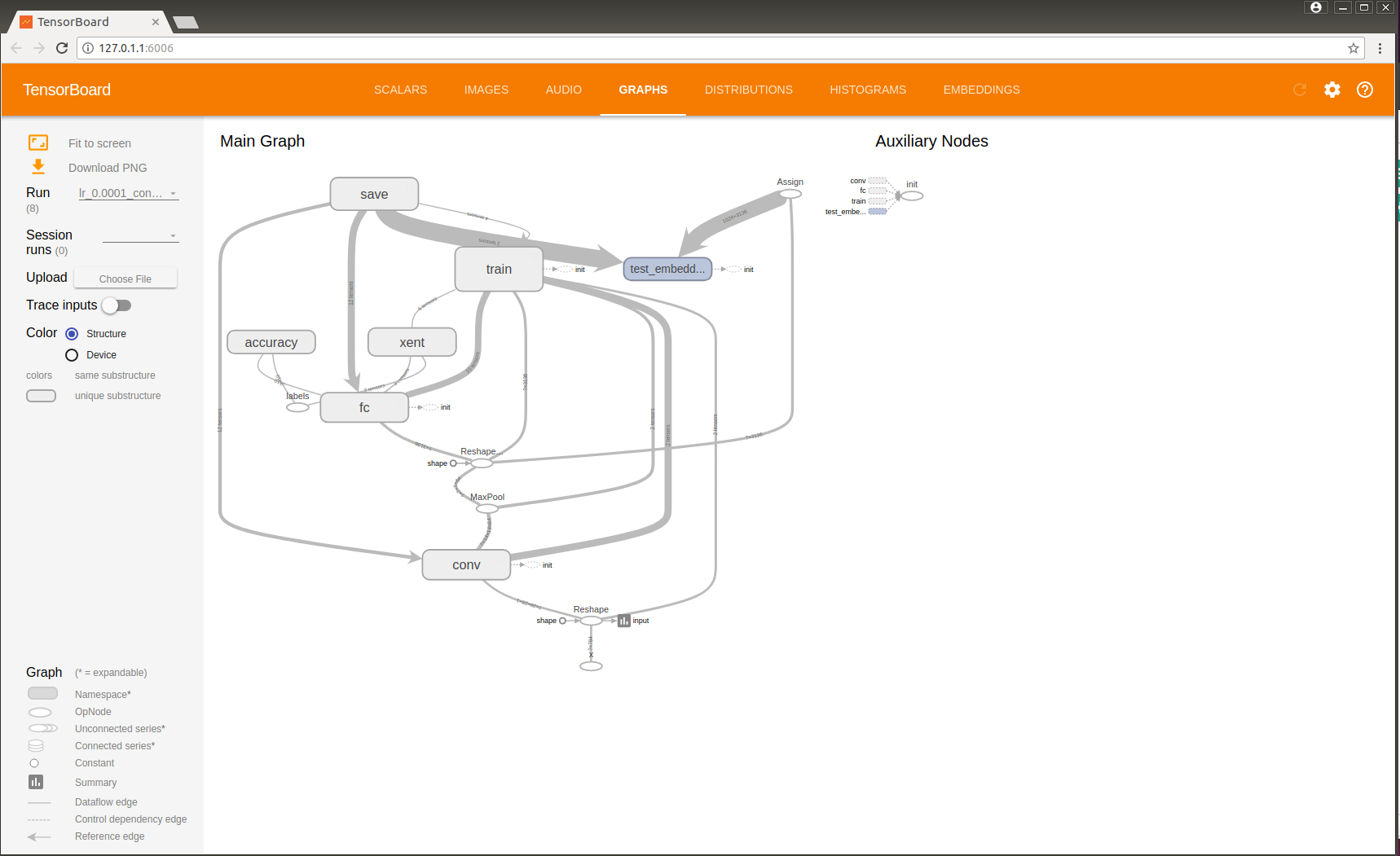
如图展示了不同模型的结构,可以用Run分别展示每个模型。有相似结构的block会有同样的color,如果既用了cpu也用了 gpu,点上color by device就会有不同颜色。打开 trace inputs,就可以看到你选中的变量,都与哪些变量有关。
看我写的辛苦求打赏啊!!!有学术讨论和指点请加微信manutdzou,注明